


Image Super-Resolution Using Deep Convolutional Networks
6 Simple steps to go from training to deploying the model. (Getting Started)


This article is based on a method proposed in the research paper which talks about a single image deep learning method that directly learns an end-to-end mapping between the low/high-resolution images.
How is this different from traditional image learning methods? How is deep learning applied here, if you may ask, this simple illustration below could give you a brief glimpse as I intend to focus on the method itself I will not go too deep on this subject. But in short, there is a mapping involved that handles each component separately and all layers in the neural network get optimized.
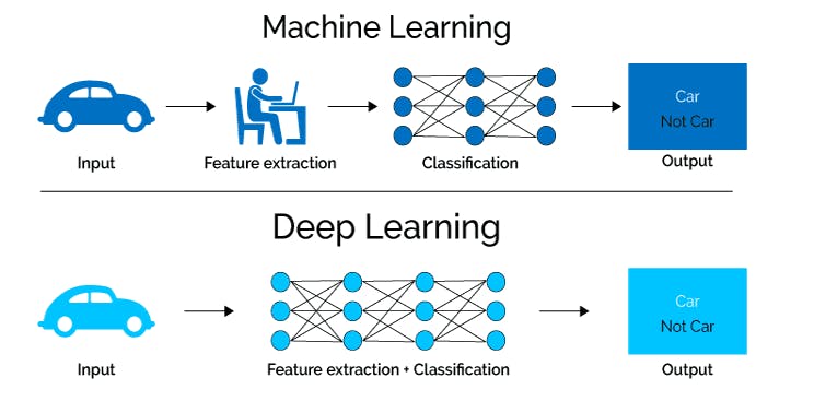
The mapping is represented as a deep convolutional neural network (CNN) that takes the low-resolution image as the input and outputs the high-resolution one.
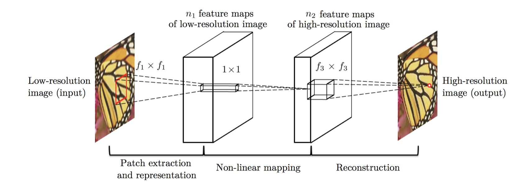
We can see in this paper that traditional sparse-coding-based SR methods can also be viewed as a deep convolutional network. But unlike traditional methods that handle each component separately, this method jointly optimizes all layers. This particular deep CNN has a lightweight structure, yet demonstrates state-of-the-art restoration quality, and achieves fast speed for practical online usage.
The goal of super-resolution (SR) is to recover a high-resolution image from a low-resolution input, or as they might say on any modern crime show, enhance!
To accomplish this goal, we will be deploying the super-resolution convolution neural network (SRCNN) using Keras. This network was published in the paper, "Image Super-Resolution Using Deep Convolutional Networks" by Chao Dong, et al. in 2014. You can read the full paper at arxiv.org/abs/1501.00092 and also passing the credit to Eduonix for the approach to problem-solving.
To evaluate the performance of this network, we will be using three image quality metrics: peak signal to noise ratio (PSNR), mean squared error (MSE), and the structural similarity (SSIM) index.
According to the image priors, single-image super-resolution algorithms can be categorized into four types – prediction models, edge-based methods, image statistical methods and patch-based (or example-based) methods. These methods have been thoroughly investigated and evaluated in Yang et al.’s work
Furthermore, we will be using OpenCV, the Open Source Computer Vision Library. OpenCV was originally developed by Intel and is used for many real-time computer vision applications. In this particular project, we will be using it to pre and post-process our images. As you may need it, we will frequently be converting our images back and forth between the RGB, BGR, and YCrCb color spaces. This is necessary because the SRCNN network was trained on the luminance (Y) channel in the YCrCb color space.
In this article, we will learn how to:
- use the PSNR, MSE, and SSIM image quality metrics,
- process images using OpenCV,
- convert between the RGB, BGR, and YCrCb color spaces,
- build deep neural networks in Keras,
- deploy and evaluate the SRCNN network
Let's get started
Step 1: Imports!
# check package versions
import sys
import keras
import cv2
import numpy
import matplotlib
import skimage

from keras.models import Sequential
from keras.layers import Conv2D
from keras.optimizers import Adam
from skimage.measure import compare_ssim as ssim
from matplotlib import pyplot as plt
import cv2
import numpy as np
import math
import os

# python magic function, displays pyplot figures in the notebook
%matplotlib inline
Step 2. Setting up Image Quality Metrics
In this step, let us write functions to calculate PSNR, MSE, and SSIM. SSIM library exists in Scikit learn, however, for PSNR and MSE we write our own functions. (Thanks Eduonix for this)
# define a function for peak signal-to-noise ratio (PSNR)
def psnr(target, ref):

    # assume RGB image
    target_data = target.astype(float)
    ref_data = ref.astype(float)

    diff = ref_data - target_data
    diff = diff.flatten('C')

    rmse = math.sqrt(np.mean(diff ** 2.))

    return 20 * math.log10(255. / rmse)

# define function for mean squared error (MSE)
def mse(target, ref):
    # the MSE between the two images is the sum of the squared difference between the two images
    err = np.sum((target.astype('float') - ref.astype('float')) ** 2)
    err /= float(target.shape[0] * target.shape[1])

    return err

# define function that combines all three image quality metrics
def compare_images(target, ref):
    scores = []
    scores.append(psnr(target, ref))
    scores.append(mse(target, ref))
    scores.append(ssim(target, ref, multichannel =True))

    return scores
Step 3:
For this project, we will be using the same images that were used in the original SRCNN paper. We can download these images from mmlab.ie.cuhk.edu.hk/projects/SRCNN.html. The .zip file identified as the MATLAB code contains the images we want. Copy both the Set5 and Set14 datasets into a new folder called 'source'.
Now that we have some images, we want to produce low-resolution versions of these same images. We can accomplish this by resizing the images, both downwards and upwards, using OpenCV. There are several interpolation methods that can be used to resize images; however, we will be using bilinear interpolation.
Once we produce these low-resolution images, we can save them in a new folder.
# prepare degraded images by introducing quality distortions via resizing

def prepare_images(path, factor):

    # loop through the files in the directory
    for file in os.listdir(path):

        # open the file
        img = cv2.imread(path + '/' + file)

        # find old and new image dimensions
        h, w, _ = img.shape
        new_height = h / factor
        new_width = w / factor

        # resize the image - down
        img = cv2.resize(img, (new_width, new_height), interpolation = cv2.INTER_LINEAR)

        # resize the image - up
        img = cv2.resize(img, (w, h), interpolation = cv2.INTER_LINEAR)

        # save the image
        print('Saving {}'.format(file))
        cv2.imwrite('images/{}'.format(file), img)
And then run the following
prepare_images('source/', 2)
The output will be
Saving baboon.bmp
Saving baby_GT.bmp
Saving barbara.bmp
Saving bird_GT.bmp
Saving butterfly_GT.bmp
Saving coastguard.bmp
Saving comic.bmp
Saving face.bmp
Saving flowers.bmp
Saving foreman.bmp
Saving head_GT.bmp
Saving lenna.bmp
Saving monarch.bmp
Saving pepper.bmp
Saving ppt3.bmp
Saving woman_GT.bmp
Saving zebra.bmp
Step 4: Time to test Low-Resolution Images
To ensure that our image quality metrics are being calculated correctly and that the images were effectively degraded, let us calculate the PSNR, MSE, and SSIM between our reference images and the degraded images that we just prepared.
# test the generated images using the image quality metrics

for file in os.listdir('images/'):

    # open target and reference images
    target = cv2.imread('images/{}'.format(file))
    ref = cv2.imread('source/{}'.format(file))

    # calculate score
    scores = compare_images(target, ref)

    # print all three scores with new line characters (\n)
    print('{}\nPSNR: {}\nMSE: {}\nSSIM: {}\n'.format(file, scores[0], scores[1], scores[2]))
the output will print to the following
baboon.bmp
PSNR: 22.1570840834
MSE: 1187.11613333
SSIM: 0.6292775879

baby_GT.bmp
PSNR: 34.3718064097
MSE: 71.2887458801
SSIM: 0.935698787272

barbara.bmp
PSNR: 25.9066298376
MSE: 500.655085359
SSIM: 0.809863264641

bird_GT.bmp
PSNR: 32.8966447287
MSE: 100.123758198
SSIM: 0.953364486603

butterfly_GT.bmp
PSNR: 24.7820765603
MSE: 648.625411987
SSIM: 0.879134476384

coastguard.bmp
PSNR: 27.1616006639
MSE: 375.008877841
SSIM: 0.756950063355

comic.bmp
PSNR: 23.7998615022
MSE: 813.233883657
SSIM: 0.83473354164

face.bmp
PSNR: 30.9922065029
MSE: 155.231897185
SSIM: 0.800843949229

flowers.bmp
PSNR: 27.4545048054
MSE: 350.550939227
SSIM: 0.869728628697

foreman.bmp
PSNR: 30.1445653266
MSE: 188.688348327
SSIM: 0.933268417389

head_GT.bmp
PSNR: 31.0205028482
MSE: 154.22377551
SSIM: 0.801112133073

lenna.bmp
PSNR: 31.4734929787
MSE: 138.948005676
SSIM: 0.846098920052

monarch.bmp
PSNR: 30.1962423653
MSE: 186.456436157
SSIM: 0.943957429343

pepper.bmp
PSNR: 29.8894716169
MSE: 200.103393555
SSIM: 0.835793756846

ppt3.bmp
PSNR: 24.8492616895
MSE: 638.668426391
SSIM: 0.928402394232

woman_GT.bmp
PSNR: 29.3262362808
MSE: 227.812729498
SSIM: 0.933539728047

zebra.bmp
PSNR: 27.9098406393
MSE: 315.658545953
SSIM: 0.891165620933
Step 5: Let's build the SRCNN Model
Now that we have our low-resolution images and all three image quality metrics functioning properly, we can start building the SRCNN. In Keras, it's as simple as adding layers one after the other. The architecture and hyperparameters of the SRCNN network can be obtained from the publication referenced above. I am following the method suggested by Eduonix.
# define the SRCNN model
def model():

    # define model type
    SRCNN = Sequential()

    # add model layers
    SRCNN.add(Conv2D(filters=128, kernel_size = (9, 9), kernel_initializer='glorot_uniform',
                     activation='relu', padding='valid', use_bias=True, input_shape=(None, None, 1)))
    SRCNN.add(Conv2D(filters=64, kernel_size = (3, 3), kernel_initializer='glorot_uniform',
                     activation='relu', padding='same', use_bias=True))
    SRCNN.add(Conv2D(filters=1, kernel_size = (5, 5), kernel_initializer='glorot_uniform',
                     activation='linear', padding='valid', use_bias=True))

    # define optimizer
    adam = Adam(lr=0.0003)

    # compile model
    SRCNN.compile(optimizer=adam, loss='mean_squared_error', metrics=['mean_squared_error'])

    return SRCNN
Step 6: Deploying the Model
Now that we have defined our model, we can use it for single-image super-resolution. However, before we do this, we will need to define a couple of image processing functions. Furthermore, it will be necessary to preprocess the images extensively before using them as inputs to the network. This processing will include cropping and color space conversions.
Additionally, to save us the time it takes to train a deep neural network, we will be loading pre-trained weights for the SRCNN. These weights can be found at the following GitHub page: github.com/MarkPrecursor/SRCNN-keras
Once we have tested our network, we can perform single-image super-resolution on all of our input images. Furthermore, after processing, we can calculate the PSNR, MSE, and SSIM on the images that we produce. We can save these images directly or create subplots to conveniently display the original, low resolution, and high-resolution images side by side.
# define necessary image processing functions

def modcrop(img, scale):
    tmpsz = img.shape
    sz = tmpsz[0:2]
    sz = sz - np.mod(sz, scale)
    img = img[0:sz[0], 1:sz[1]]
    return img


def shave(image, border):
    img = image[border: -border, border: -border]
    return img
And then:
# define main prediction function

def predict(image_path):

    # load the srcnn model with weights
    srcnn = model()
    srcnn.load_weights('3051crop_weight_200.h5')

    # load the degraded and reference images
    path, file = os.path.split(image_path)
    degraded = cv2.imread(image_path)
    ref = cv2.imread('source/{}'.format(file))

    # preprocess the image with modcrop
    ref = modcrop(ref, 3)
    degraded = modcrop(degraded, 3)

    # convert the image to YCrCb - (srcnn trained on Y channel)
    temp = cv2.cvtColor(degraded, cv2.COLOR_BGR2YCrCb)

    # create image slice and normalize
    Y = numpy.zeros((1, temp.shape[0], temp.shape[1], 1), dtype=float)
    Y[0, :, :, 0] = temp[:, :, 0].astype(float) / 255

    # perform super-resolution with srcnn
    pre = srcnn.predict(Y, batch_size=1)

    # post-process output
    pre *= 255
    pre[pre[:] > 255] = 255
    pre[pre[:] < 0] = 0
    pre = pre.astype(np.uint8)

    # copy Y channel back to image and convert to BGR
    temp = shave(temp, 6)
    temp[:, :, 0] = pre[0, :, :, 0]
    output = cv2.cvtColor(temp, cv2.COLOR_YCrCb2BGR)

    # remove border from reference and degraged image
    ref = shave(ref.astype(np.uint8), 6)
    degraded = shave(degraded.astype(np.uint8), 6)

    # image quality calculations
    scores = []
    scores.append(compare_images(degraded, ref))
    scores.append(compare_images(output, ref))

    # return images and scores
    return ref, degraded, output, scores
and then:
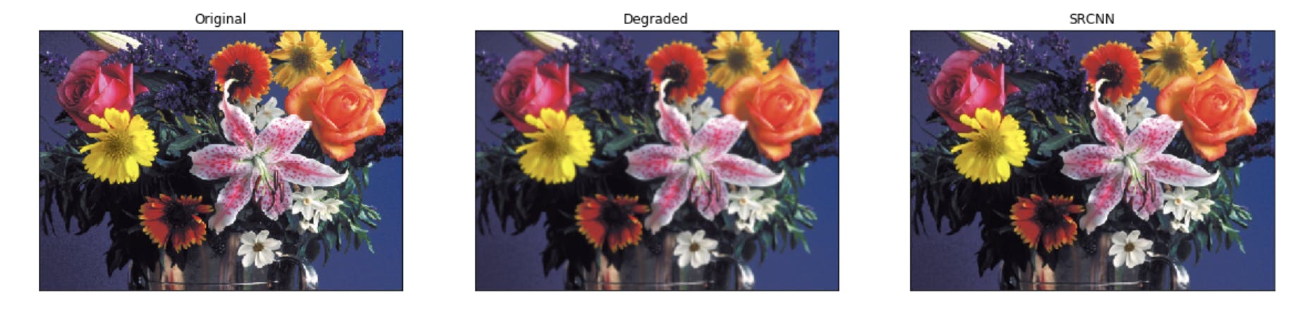
ref, degraded, output, scores = predict('images/flowers.bmp')

# print all scores for all images
print('Degraded Image: \nPSNR: {}\nMSE: {}\nSSIM: {}\n'.format(scores[0][0], scores[0][1], scores[0][2]))
print('Reconstructed Image: \nPSNR: {}\nMSE: {}\nSSIM: {}\n'.format(scores[1][0], scores[1][1], scores[1][2]))


# display images as subplots
fig, axs = plt.subplots(1, 3, figsize=(20, 8))
axs[0].imshow(cv2.cvtColor(ref, cv2.COLOR_BGR2RGB))
axs[0].set_title('Original')
axs[1].imshow(cv2.cvtColor(degraded, cv2.COLOR_BGR2RGB))
axs[1].set_title('Degraded')
axs[2].imshow(cv2.cvtColor(output, cv2.COLOR_BGR2RGB))
axs[2].set_title('SRCNN')

# remove the x and y ticks
for ax in axs:
    ax.set_xticks([])
    ax.set_yticks([])
Output will be
Degraded Image:
PSNR: 27.2486864596
MSE: 367.564000474
SSIM: 0.86906220246

Reconstructed Image:
PSNR: 29.6675381755
MSE: 210.594874985
SSIM: 0.899043290319
Now for the rest of it we can save the images
for file in os.listdir('images'):

    # perform super-resolution
    ref, degraded, output, scores = predict('images/{}'.format(file))

    # display images as subplots
    fig, axs = plt.subplots(1, 3, figsize=(20, 8))
    axs[0].imshow(cv2.cvtColor(ref, cv2.COLOR_BGR2RGB))
    axs[0].set_title('Original')
    axs[1].imshow(cv2.cvtColor(degraded, cv2.COLOR_BGR2RGB))
    axs[1].set_title('Degraded')
    axs[1].set(xlabel = 'PSNR: {}\nMSE: {} \nSSIM: {}'.format(scores[0][0], scores[0][1], scores[0][2]))
    axs[2].imshow(cv2.cvtColor(output, cv2.COLOR_BGR2RGB))
    axs[2].set_title('SRCNN')
    axs[2].set(xlabel = 'PSNR: {} \nMSE: {} \nSSIM: {}'.format(scores[1][0], scores[1][1], scores[1][2]))

    # remove the x and y ticks
    for ax in axs:
        ax.set_xticks([])
        ax.set_yticks([])

    print('Saving {}'.format(file))
    fig.savefig('output/{}.png'.format(os.path.splitext(file)[0]))
    plt.close()
That will output to:
Saving baboon.bmp
Saving baby_GT.bmp
Saving barbara.bmp
Saving bird_GT.bmp
Saving butterfly_GT.bmp
Saving coastguard.bmp
Saving comic.bmp
Saving face.bmp
Saving flowers.bmp
Saving foreman.bmp
Saving head_GT.bmp
Saving lenna.bmp
Saving monarch.bmp
Saving pepper.bmp
Saving ppt3.bmp
Saving woman_GT.bmp
Saving zebra.bmp
Thus we now have a model that could use Super-Resolution Convolutional Neural Network (SRCNN) surpasses the bicubic baseline with just a few training iterations and outperforms the sparse-coding-based method (SC) with moderate training. The performance may be further improved with more training iterations.
Hope you enjoyed the post. Please share/subscribe or connect with me for more on Linkedin